Top Memory Bandwidth Guide: How Does It Work?
How memory bandwidth works becomes clearer when we follow each data transfer. Memory bandwidth describes how much information memory can deliver per second. It is usually measured in gigabytes per second. A simple estimate multiplies the transfer rate, bus width, and number of memory channels. For example, DDR5-5600 transfers 5.6 billion data units per second. A 64-bit channel moves eight bytes per transfer. Multiple channels increase the available path.
The concept also explains why modern processors need wider, faster memory systems. David Patterson, a leading computer architect, described the central problem this way: “The memory wall is the gap between processor speed and memory speed.” His statement remains useful. A processor may finish calculations quickly, then wait for data from memory. That pause can reduce real performance. GPUs, servers, and integrated graphics often expose this limitation more clearly than ordinary desktops.
Bandwidth is not the same as latency. Bandwidth measures flow. Latency measures waiting time. Cache size, access patterns, memory rank, and channel configuration all affect results. Dual-channel memory can outperform single-channel memory, even with identical modules. The improvement depends on the workload. Video rendering benefits strongly. Small office applications may show little change.
Benchmarks reveal the practical difference. A memory test might report 80 GB/s, while an application uses far less. The number is theoretical. That matters. Cooling, firmware settings, and background processes can also change measurements. This guide examines the calculation, hardware pathway, testing methods, and upgrade choices. It also questions a common assumption: more bandwidth does not automatically mean a faster computer.
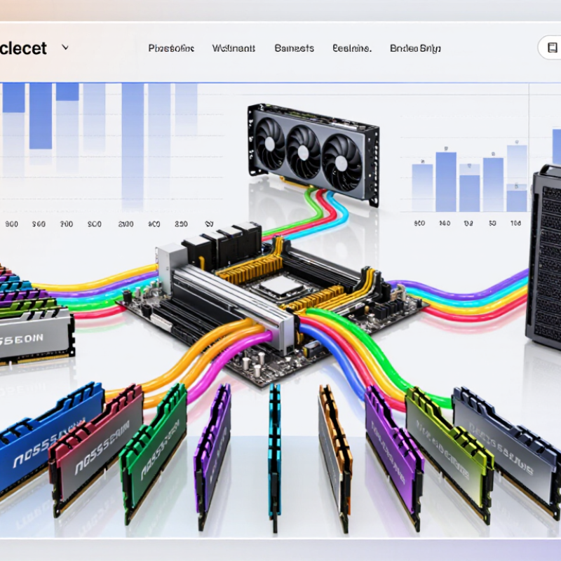
Top Memory Bandwidth Guide: How Does It Work?
Memory bandwidth means the amount of data a memory system can move each second. It is different from storage capacity. Capacity is the size of the room; bandwidth is the width of the doorway. A common formula is simple: transfers per second multiplied by bus width, divided by eight. Under the JEDEC JESD79-5C specification, DDR5-6400 can reach 51.2 GB/s on one 64-bit channel.
That figure describes theoretical peak performance. Real workloads often achieve less. Latency, memory-controller scheduling, thermal limits, and competing threads all reduce usable bandwidth. I used to treat the advertised number as practical speed. That was too optimistic. A processor reading scattered data may leave much of the channel idle, even with fast memory installed.
High-performance systems use wider interfaces. JEDEC’s HBM3 specification supports up to 6.4 gigatransfers per second across a 1,024-bit interface, producing about 819.2 GB/s per stack. This helps data-heavy workloads, including scientific simulation and large model training. However, bandwidth alone cannot fix poor software locality. The 2024 TOP500 list also shows why system design matters: leading systems combine processors, memory, interconnects, and cooling rather than relying on one specification. The number looks impressive. The bottleneck may sit elsewhere.
| Memory Technology or Configuration | Typical Data Rate | Effective Bus Width | Theoretical Bandwidth | Calculation Example | Common Workload Characteristics |
|---|---|---|---|---|---|
| DDR4-2400, single 64-bit channel | 2,400 MT/s | 64 bits / 8 bytes | 19.2 GB/s | 2,400 × 8 ÷ 1,000 = 19.2 GB/s | General-purpose computing with moderate memory-transfer requirements. |
| DDR4-3200, single 64-bit channel | 3,200 MT/s | 64 bits / 8 bytes | 25.6 GB/s | 3,200 × 8 ÷ 1,000 = 25.6 GB/s | Desktop and server workloads requiring a balanced combination of capacity, latency, and bandwidth. |
| DDR4-3200, dual-channel configuration | 3,200 MT/s per channel | 128 bits / 16 bytes total | 51.2 GB/s | 25.6 GB/s × 2 channels = 51.2 GB/s | Applications that benefit from parallel memory channels, including content creation and multitasking. |
| DDR5-4800, single 64-bit channel | 4,800 MT/s | 64 bits / 8 bytes | 38.4 GB/s | 4,800 × 8 ÷ 1,000 = 38.4 GB/s | Modern computing systems with increased data-transfer demand and improved memory parallelism. |
| DDR5-5600, single 64-bit channel | 5,600 MT/s | 64 bits / 8 bytes | 44.8 GB/s | 5,600 × 8 ÷ 1,000 = 44.8 GB/s | High-performance desktop and workstation workloads with substantial memory traffic. |
| DDR5-5600, dual-channel configuration | 5,600 MT/s per channel | 128 bits / 16 bytes total | 89.6 GB/s | 44.8 GB/s × 2 channels = 89.6 GB/s | Parallel workloads, integrated graphics, simulation, compilation, and professional applications. |
| LPDDR5-6400, single 64-bit interface | 6,400 MT/s | 64 bits / 8 bytes | 51.2 GB/s | 6,400 × 8 ÷ 1,000 = 51.2 GB/s | Power-efficient mobile and thin-system designs that require high bandwidth within a limited energy budget. |
| GDDR6, 16 Gb/s with a 256-bit bus | 16 Gb/s per pin | 256 bits / 32 bytes | 512 GB/s | 16 × 256 ÷ 8 = 512 Gb/s = 512 GB/s | Graphics and parallel processors that need much higher throughput than ordinary system memory. |
| GDDR6, 16 Gb/s with a 384-bit bus | 16 Gb/s per pin | 384 bits / 48 bytes | 768 GB/s | 16 × 384 ÷ 8 = 768 Gb/s = 768 GB/s | High-throughput graphics workloads involving large textures, frame buffers, and parallel calculations. |
| HBM2e, one 1,024-bit stack | 3.2 Gb/s per pin | 1,024 bits / 128 bytes | 409.6 GB/s | 3.2 × 1,024 ÷ 8 = 409.6 GB/s | Compute accelerators and graphics processors designed for very wide, energy-efficient memory interfaces. |
| HBM3, one 1,024-bit stack | 6.4 Gb/s per pin | 1,024 bits / 128 bytes | 819.2 GB/s | 6.4 × 1,024 ÷ 8 = 819.2 GB/s | Artificial intelligence, high-performance computing, scientific modeling, and bandwidth-intensive acceleration. |
Memory bandwidth is the amount of data memory can transfer each second. It measures capacity, not waiting time. Think of it as a data road.
Use this formula: bandwidth equals transfer rate multiplied by bus width, divided by eight. The division changes bits into bytes.
Memory running at 3,200 MT/s with a 64-bit bus provides 25,600 MB/s. That equals about 25.6 GB/s. The figure is theoretical.
MT/s means millions of transfers per second. It does not mean megahertz. A 1,600 MHz clock can produce 3,200 MT/s with double-data-rate memory.
Two active channels can nearly double the theoretical result. For example, 25.6 GB/s may become 51.2 GB/s. Both channels must operate correctly.
No. Processor cache, storage access, software design, and latency can limit performance. My early assumption was too simple. More bandwidth is not always the answer.
Timing, controller efficiency, scattered requests, and competing tasks reduce real performance. A large-array workload may approach the limit. Small applications may barely use it.
Measure sustained bandwidth during the actual task, not only a synthetic benchmark. Watch memory use, processor activity, and access patterns together. Results need context.
Some tools use decimal units, while others use binary units. Their numbers may look inconsistent. Check the unit definition before comparing results.
Memory bandwidth describes how much data a computer’s memory system can transfer to and from the processor within a given period. How memory bandwidth works depends on factors such as the transfer rate, data bus width, number of memory channels, and the timing of each operation. A common theoretical calculation multiplies the transfer rate by the bus width and divides the result by eight to express capacity in bytes per second.
Data moves through coordinated paths between memory modules, memory controllers, caches, and the processor. Although high theoretical bandwidth can support faster data movement, real performance also depends on latency, access patterns, workload size, and whether multiple components compete for memory access. Hardware design, channel configuration, clock speed, and system limits all influence the final result. Performance can be evaluated with memory benchmarks and practical applications, while improvements may come from better configuration, efficient software, reduced unnecessary data transfers, and balanced memory settings.

 Kryntel